PscanChIP Help
Input
Example: submitting ChIP-Seq enriched regions
Example: submitting ChIP-Seq enriched regions and matrices
Output
Performing a motif-centered analysis
Reading p-values
Sample data sets
Resetting the interface
PscanChIP is a web application that, given a set of genomic regions derived from a genome wide ChIP-Seq experiment, scans them and looks for over represented sequence motifs, according to motif descriptors of the TRANSFAC and JASPAR databases, or uploaded by users. The over represented motifs thus correspond to transcription factor binding sites found to be enriched in the regions themselves. Over representation is assessed with different strategies (see Output), that take advantage of the high resolution that modern ChIP-Seq can offer. Also, output from experiments like ChIP-exo are perfectly suitable for PscanChIP, in order to discover binding sites correlations and preferential arrangements. The general idea is to assess which is the motif more likely to represent the binding specificity of the TF investigated; but also to identify "secondary" motifs which might correspond to other TFs interacting with the one for which the ChIP experiment was performed.
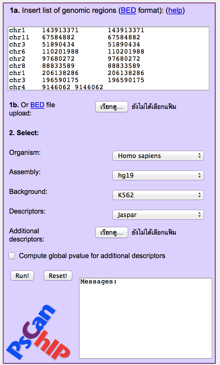
Input:
Just submit a list of genomic coordinates in BED format, which basically consists of three elements per line:
chromosome start end
You can either paste the coordinates in the text box, or load a text file. The program checks whether each line starts with these three elements. Additional elements after the end coordinates will be automatically ignored keeping the coordinates only. Lines not complying with this format, or containing inconsistent genomic coordinates will be automatically ignored (and reported in the text box at the bottom once the analysis has been started.
It is essential that genomic coordinates correspond to ChIP-Seq enriched regions centered around their summits, that is, centered on the point of maximum within the "peak". Regions do not have to be of the same size, and can be of any size. The program will assume they are centered around the point of local maximum of a ChIP-Seq peak and will analyse the 150 bp around that point. Thus, if a input region is shorter, it will be extended on both sides of the same number of bps until it is 150 bp long. If longer, it will be trimmed on both sides of the same number of bp to yield a 150 bp region. There is no maximum number of regions that can be input.
Optionally, you can input the regions sorted in decreasing order according to their enrichment and/or significance p-value (the most enriched at the top), in order to assess also the correlation between the enrichment of a motif and the enrichment of the regions in the ChIP-Seq (see the Output section).
The input parameters that have to be set are the organism (human or mouse) and the genome assembly to be used (make sure it matches the genome assembly that was used for the ChIP-Seq analysis).
In the background field you can select the genomic background to be used to assess global enrichment of motifs (see the Output section). It is computed on human cell lines for which DNaseI digital genomic footprinting data are already available. These kind of data are used to identify sites where regulatory factors bind to the genome (footprints). If the cells/tissue on which your ChIP-Seq experiment was performed is not on the list, you can either choose what seems the closest one (e.g. HepG2 for liver cells), or select the "mixed" background, built using a random selection of regions from different cells. Alternatively, if your ChIP-Seq regions are restricted to or mostly come from gene promoters, you can select "Promoters" as a background.
You may find a summary description of cell/tissue types
here.
With the "Select Descriptors"
option you can choose whether the analysis has to be performed with
the TFBSs matrices available in the JASPAR or TRANSFAC databases, or
if you want to upload a specific matrix set which will be added to
the chosen database. In the latter case, prepare
a TEXT file containing one or more matrices in the following format:
>matrix1
A_1 A_2 ..... A_n
C_1 C_2 ..... C_n
G_1 G_2 ..... G_n
T_1 T_2 ..... T_n
>matrix2
A_1 A_2 ..... A_n
C_1 C_2 ..... C_n
G_1 G_2 ..... G_n
T_1 T_2 ..... T_n
..and so on, where A_i, etc. are the frequencies of the four nucleotides in the
columns of the matrix. These values can be either integers or floating
point values, they will be automatically rescaled to frequencies summing
to one in each column. There's an example matrix file in the main page.
Each matrix is preceded by a "fasta-like" line containing its name.
Notice that matrix names can contain only letters or digits, and every
matrix has to have a different name. Up to 50 matrices can be uploaded.
Submitting ChIP-Seq enriched regions
On the right-hand column of the main page several datasets are available
for testing the interface. Clicking on any link automatically loads a list
of genomic coordinates in the input text box.
For example, click on the NF-YA link. It contains a set of regions of the ENCODE
project enriched for the binding of the YA subunit of NF-Y in the K562 cell line.
As you can notice, the regions are of 1 bp, matching exactly the point of local maximum
(summit) of the peaks. They will be automatically extended by 75 bp in each direction,
yielding for the analysis 150 bp regions.
Below the input box, you can choose the source organism (human, in this
case), the genome assembly (hg19), the cell line (K562, included in the list)
and the
matrix database you want to use (Jaspar, Transfac, or you can upload one
or more matrices). For the example, all these parameters have been automatically set.
Click "Run!"
In the textbox under the "Run" button, a confirmation message has appeared. Any
wrongly formatted region in the input will be reported in the textbox, as well
as genomic coordinates not matching the genome assembly selected. Note: a
large number of regions on "normal" chromosomes of the assembly reported as wrong and discarded
is a likely indicator
that you selected the wrong genome/assembly as input.
Results will shortly appear in the middle column of the page (see the Output section).
Similar experiments can be performed with all the other input sets provided (all parameters are set automatically), except for Sample 3 for which a user-defined matrix has to be uploaded, as explained in the next section.
Submitting ChIP-Seq enriched regions and matrices
As an example of user-defined matrices, we included the NRF1 binding site
matrix, since it is not included in the TRANSFAC matrices publicly available at the time of the release of PscanChIP.
Also, this is what can be done if, for example, a motif finding tool has been run on the regions beforehand, and one or more matrices have been built as a result.
The matrix is contained in this file. Save it on your
computer. In the input page, load the set of NRF1 enriched regions in hESC cells by clicking the corresponding link.
Then, click on the "Choose File" (or similar messages, according to the browser you use) button next to the "Additional descriptors" textbox, and locate the file containing
the NRF1 matrix you just saved.
If you want PscanChIP to compute global enriched p-values also for the matrices you uploaded, check the "Compute global pvalue for additional descriptors" at the bottom of the parameter list. The downside is that the computation time can be expected to take from 2 to 5 minutes more than a run without this option. The bright side is obviously that you will get a very useful piece of information (global p-values) also for user defined matrices.
Finally, click on "Run".
Once again, the results will appear in the middle column (otherwise, in case
of any problem with the matrix file an error message will appear in the
text box under the "Run" button).
Everything now is the same as in the previous
example (see the Output section), with the exception that the matrices
you uploaded are added to the matrix set chosen (JASPAR or TRANSFAC) and will appear
togeter with them in the summary table. The name of the user-submitted matrices is read from the uploaded file (in the line starting with the '>' symbol), and preceded by the prefix "UMAT_". If the "global p-value" option for user defined matrices was not checked, the global p-value field for these will be left empty. In the NRF1 example, thus, in the results the matrix uploaded will be named "UMAT1_NRF1". Matrix names can contain only letters or digits, and every matrix has to have a different name. Up to 25 matrices can be uploaded.
Output:
When you click the "Run" button, a confirmation message (with possible warnings about the input) appears
in the text box next to it.
The result of the computation will appear in
the middle column of the page. The figure shows the output for the NF-Y/K562 example (sample 1).
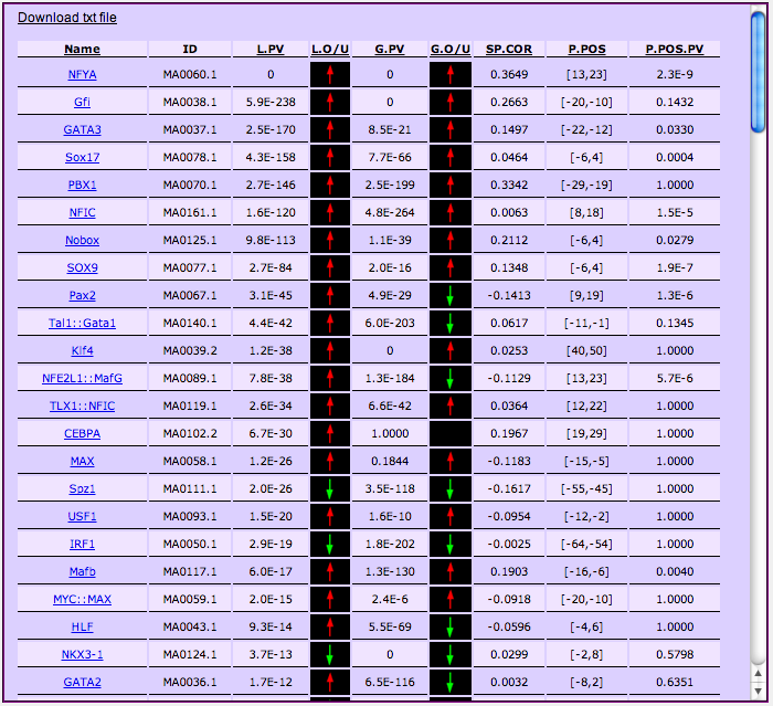
For each matrix (including those you uploaded, if any), PscanChIP computes an enrichment P-value according to three different criteria. More in detail, from left to right, each line of the output table corresponds to a matrix, and it contains the following information:
- Name and ID: the name and the database ID of the matrix.
- Local enrichment p-value (L.PV): describing if the matrix is over- or under-represented in the 150 bp input regions with respect to the genomic regions flanking them. Since the p-value is computed with a two sided t-test, next to the p-value an arrow (L.O/U) indicates whether it means that the matrix motif tends to be over-represented in the sample (red arrow pointing upwards) or vice versa avoided (green arrow pointing downwards).
-
Global enrichment (G.PV), describing if the matrix is over- or under-represented in the input regions with respect to a global background made of a genome-wide collection of putative regulatory (TF accessible) regions in various cell lines. Once again, the p-value is computed with a two sided t-test, next to the p-value an arrow (G.O/U) indicates whether the matrix motif tends to be over-represented in the sample (red arrow pointing upwards) or vice versa avoided (green arrow pointing downwards). This value is computed for user-submitted matrices only if the "Compute global pvalue for additional descriptors" options was set at input.
-
Spearman correlation coefficient (SP.COR): if the input regions were ranked according to their enrichment, this value represents the Spearman rank correlation coeffifient between the ranking of the input regions and their ranking with respect to the motif. In other words, positive values indicate that the more enriched regions are, the best matches they contain for the motif. A correlation around zero denotes no significant correlation, while a negative value is an indicator of anti-correlation (i.e. the more enriched are the regions the worse are motif matches in the regions). If your regions are *not* sorted according to enrichment, this correlation clearly has no meaning.
- Preferred position (P.POS) and position bias pvalue (P.POS.PV): this indicates the position within the regions where the motif tends to be found more frequently with best matches to the matrix. Coordinates are relative to the center of the regions, which has coordinate 0 . The associated p-value indicates the significance of the positional bias of the motif, computing both according to the number of occurrences of the motif within the region and their score. In a ChIP-Seq experiment, the matrix corresponding to the binding sites of the TF investigated should be found with low p-values at the center of the regions. But, the same holds true (positional bias) also for the TFs binding in association with the main one, as also shown by performing motif-centered analyses.
The table can be sorted according to any column value by clicking on the corresponding header. Hovering with the mouse pointer on each header will pop up a brief explanation of its meaning.
At the top of the table, "Download txt file" permits to download the results table in tab-delimited text format.
The figure above shows the output of the NF-YA sample set. It can be seen how the corresponding matrix has p-value virtually zero for local and global enrichment, and also a positive Spearman correlation and a positional bias next to the center of the regions - all indicators that this is indeed the matrix describing sites bound by NF-Y. The slight shift from the exact center of the regions might have indeed a biological meaning, since the actual NF-Y subunit binding DNA is YB and not YA.
By clicking on a matrix name (NFYA in the example), you can open a dedicated page
showing the detailed results regarding the
matrix, and in particular 1) the matrix itself, its logo (at the bottom), its information
content and links to
its database entry as well as to the ID (PMID) of the PubMed entry describing its generation.
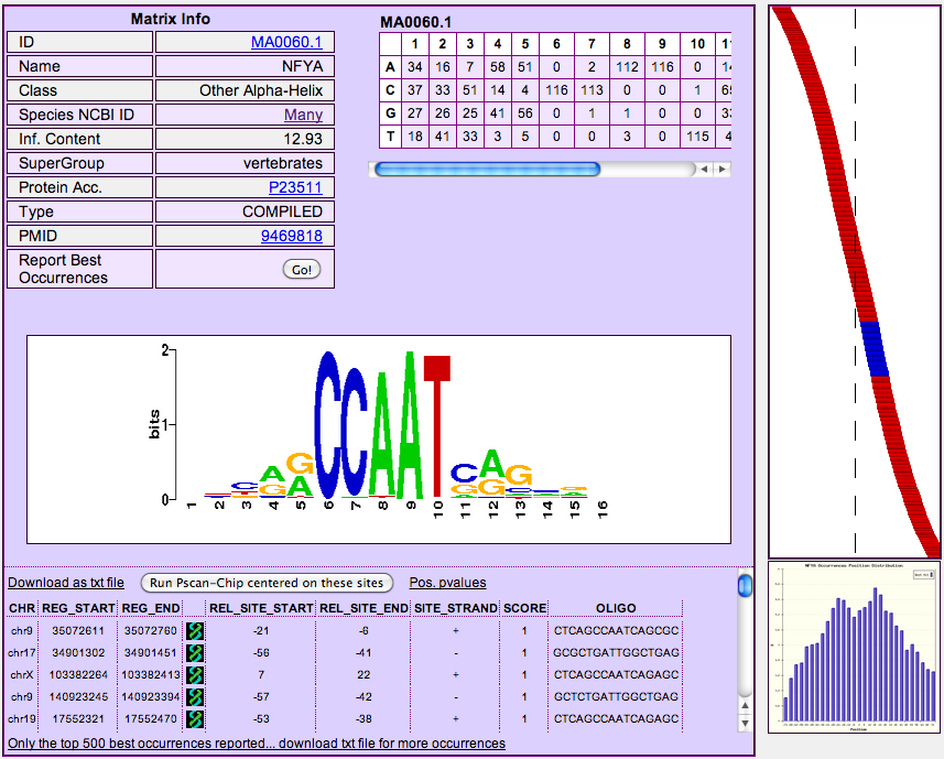
By clicking on the "Report Occurrences" button at the bottom of the "Matrix
Info" table you can retrieve, for each region submitted, the best matching
oligo in each one, as well as its score (from 0 to 1) and its position and strand,
with respect to the region itself (REL_SITE_START and REL_SITE_END, where 0 is the center of the region), and the genomic coordinates of the region (REG_START and REG_END). Clicking
the green/black UCSC logo next to the coordinates will open a page of the UCSC
genome browser showing the exact location of the region in the genome.
Occurrences are sorted according to their
score. The links above and below the occurrence table (limited to the best 500) allow you to download the complete
table in text format. On the right hand side of the page
it also appears a simple graphical representation of the location of
the best matching oligos within the regions, giving a quick view on whether, apart
from p-value calculations, there is a visible bias towards the center or any other position of the regions themselves. Oligos falling within the preferred position range (see point 5 above) are highlighted in blue.
Also, another button ("Run Pscan-Chip centered on these sites") appears above the occurrence table, allowing to start a new analysis of the same genomic
regions, but in this case centered on the occurrences reported for this motif, and not on the middle of the regions, as explained in the following section.
Performing a motif-centered analysis
A motif centered analysis can be started after a normal analysis, from the detailed output page of the matrix of interest, as explained in the precious section.
That is, you have to make Pscan report the occurrences of the motif. Then, you can click on the "Run Pscan-Chip centered on these sites" button.
The program will collect the absolute genomic coordinates of the best match for the matrix in the original regions, and extend them producing 150 regions as with ChIP-Seq summit regions. In this case, thus, coordinate 0 of each region will correspond to the center of the motif selected. A new window will open and the analysis will be started automatically.
The rationale behind this kind of analysis is that, once the binding motif for the TF investigated has been detected, further information can be gathered by re-running the analysis centered on the motif itself, so to discover at a glance whether there exist any significant positional correlation between the motif chosen and the other TRANSFAC, JASPAR or user submitted matrices, and if the correlation is significant from a statistical point of view. In this way, additional candidate TFs binding in a cooperative way (e.g. forming heterodimers) can be discovered.
The output of the motif-centered analysis is identical to the default one, with the sole difference that for the matrix chosen (whose sites will fall exactly in the middle of the regions analysed) PscanChIP will look for the second best match within the regions themselves, in order to detect if there is a preferential arrangements of sites for the same TF, e.g. in case of TFs binding as homodimers.
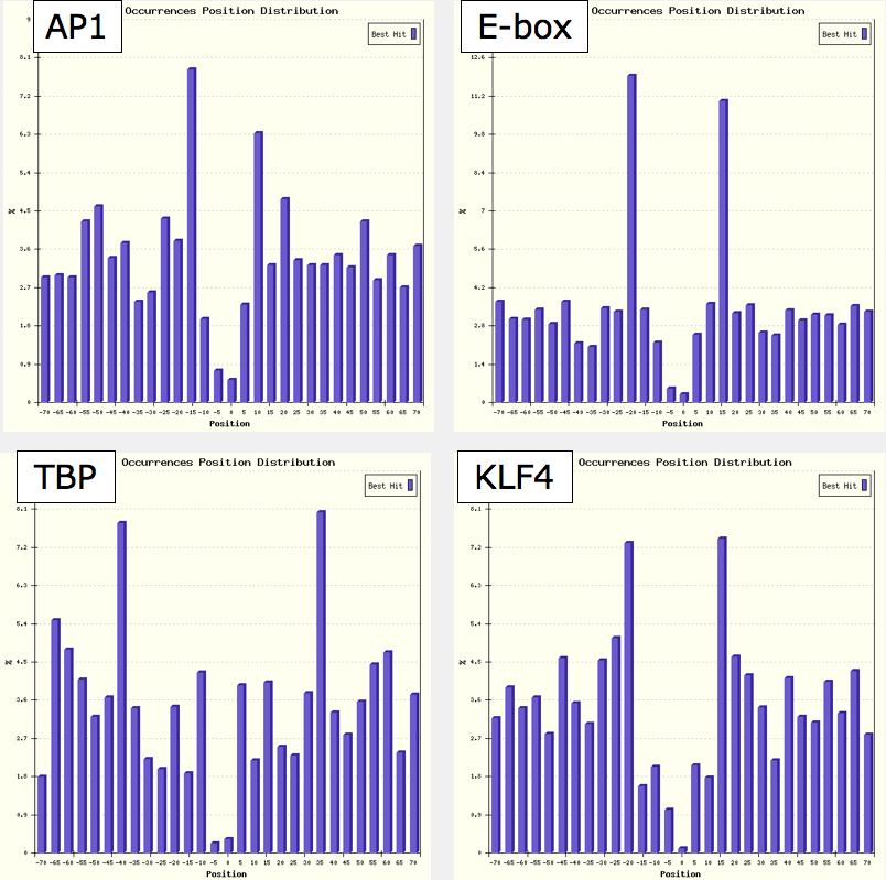
Also, above the Output table, you will find an additional link called Distance hotspots map that opens a graphical representation of the "preferred" positions of the matrices used with respect to the one on which the analysis is centered, that can be browsed (try hovering with the mouse on the red spots in the map).
For example, performing an analysis centered on the NF-Y matrix, you will notice in the result table a large number of different matrices having positional preference (P.POS) not only for the middle of the regions (as for NF-Y itself, since the analysis is exactly centered on its sites, and other factors binding CCAAT-like elements), but also with strong bias and low p-values for different portions, as for example AP1 (FOS+JUN complex), KLF4 (or Sp1), TBP, and E-box motifs (Myc, MAX, Usf1), as shown by their respective occurrence distribution plots (the dotted line correspond to the position of the NF-Y CCAAT motif):
Reading p-values: when a result is significant?
The program associates with each motif three different p-values, which imply different things and are meant to detect different levels of correlation.
Clearly, if the TF for which the ChIP was performed has its preferred binding site motif, then the corresponding matrix should present very low (usually, the lowest) p-values for global enrichment (if a region is accessible by the TF and contains the motif, then its is bound and is enriched in the ChIP; accessible regions that do not contain the motif are not bound by the TF and are not enriched in the ChIP); for local enrichment (if a region is bound by the TF, then the TF should bind close to the ChIP enrichment peak summit); for positional bias (same for local enrichment, but the resolution of ChIP-Seq is high enough to localize the actual binding sites very close to the peak summit).
Other TFs which in general can be consider co-regulators with the IP'ed TF should present a low global p-value as well, meaning than they tend to bind the same regions of the main TF (e.g. the same promoters or enhancers), but not necessarily in very close proximity. The mouse stem cell and the STAT3 datasets are an example. In the original experiments on mouse stem cells for 13 different TFs, c-Myc for example was shown to correlate with Zfx, n-Myc, Klf4 and E2F1, but not with Nanog, Sox2, Oct4, Samd1, and Stat3. This is clearly shown in the global p-value ranking, which has the matrices for the four correlating factors with low p-values, while for example matrices for Sox2 and Stat3 seem to be avoided. The correlating factors, however, do not seem to present any significant co-localization with the c-Myc profile, e.g. they might bind the same set fo promoters/enhancers but not necessarily next to it. Vice versa, in the Oct4 example, we can see enriched both locally and globally the Oct-binding profiles, and the Sox2 profile (using Jaspar matrices), confirming the physical interaction between the two factors binding as heterodimers reported in the study (see Chen et. al, Cell 2008 for a comparison of the results obtained with PscanChIP).
TFs which may interact with the IP'ed TF should still present a low local p-value, meaning that when they happen to bind the same region, they tend to bind in the neighbourhood of the main TF, but not necessarily in every or most of the regions (for this you have to check the global p-value first); TFs which also present a positional bias (with low associated p-values) can be considered again interactors of the main TF, i.e., when they bind together with the main TF they require a precise arrangement of sites hinting at physical interaction, for example, they are members of the same TF complex, but this does not imply that it happens as a rule (check the global p-value or local p-values for this). The NF-YA example previously described is a perfect case study for this. Global and local p-values show, other than NF-Y itself, a large number of over-represented matrices, unsurprisingly for a "key" factor like this. But, the motif centered analysis also shows that for several matrices there is a significant positional bias, centered like the NF-Y motif (corresponding to TFs which bind similar sequence elements), but also with significant positional bias far away from the center, as
in the examples described above.
Sample data sets
Several sample datasets are included in PscanChIP, to show different ways in which it can be applied to the analysis of regions from ChIP-Seq experiments. See also the previous section for further information on how to read the ouput, and the article for further discussion on the results.
- NF-YA ChIP-Seq in K562 human cells, assembly hg19. Shows how the binding sites for the factor investigated can be easily found over-represented in the center of the regions, with positive Spearman correlation coefficient with the input regions, which were sorted according to their enrichment. There is a large number of other motifs over-represented, either locally or globally. Performing a motif centered analysis on the NFYA matrix shows several other matrices with a precise positional preference around it (AP1, TBP, SP1, KLF4,E-box motifs like MYC, USF1, MAX, and so on) .
- 13 "core" TFs in mouse stem cells, assembly mm10. Usually, the binding sites for the factor investigated can be easily found over-represented in the center of the regions (see the article for discussion on E2F1). The global p-value enrichment is able to detect other TFs which have been demonstrated to correlate with the main one in mouse stem cells, while others not correlating have p-values pointing to the fact that their sites seem to be avoided either locally or globally in the regions.
- Sample 3 - Stat3 in four mouse cell types (sorted). Binding of Stat3 can be inferred in all the experiments, with different co-factors and interactors appearing in each dataset.
- Sample 4 - E2F1 summits in HeLa-S3 cells. "Canonical" sites for E2F1 appear to be enriched in the dataset, despite other studies suggesting the opposite (lack of sites in E2F1-bound regions). Notice however how E-box binding motifs (like Mycn) virtually present the same type of enrichment, suggesting their possible role in recruiting E2F1, at least in some contexts.
- NRF1 ChIP-Seq in hESC human cells, assembly hg19. The NRF1 matrix is not included in the TRANSFAC or JASPAR datasets, and it has to be uploaded to the interface. This is what can be done if, for example, a motif finding tool has been run on the regions beforehand, and one or more matrices have been built as a result. Running PscanChIP on them will permit to show their positional bias in the regions, and how they compare and/or correlate with other existing motif descriptors.
Resetting the interface
At any moment, you can return to the initial web page (with empty input
boxes and no results in the middle column) by clicking the "Reset" button
at the bottom of the left-hand column (next to "Run!").